
In some of my previous posts, I have discussed a few things related to time series data. However, I haven’t covered one of the most popular topics: forecasting. Even as kids, most of us were already familiar with it. At the very least, I have wished that the next day is sunny, so I could go out with my friends.
This post aims to be an introductory material to some variations of forecasting problems and approaches, without giving in-depth details of the algorithms.
What is forecasting?
As displayed in Figure 1, forecasting refers to the act of predicting future events. While “prediction” may sound more like a classification task, forecasting focuses on estimating a continuous outcome.
You may think “then, why is it called ‘weather forecast’?”. I don’t know the actual answer, but I found a possible explanation a few months ago (maybe I’m too slow in my thinking, lol). While we tend to look at the output of a weather forecast as a category (e.g., sunny, cloudy, or rainy), that category is derived based on other factors, such as wind speed, temperature, and humidity. Presumably, meteorologists forecast these factors individually (which have a continuous outcome), then they process them further and come up with the final category to simplify the interpretation. If someone knows the actual answer, please leave let me know!
Anyway, since forecasting produces a continuous outcome, sometimes it is approached as a regression problem. However, there is a key difference: there is a temporal dependence in time series data, whereas regression approaches assume that each observation is independent of the other. Despite this assumption, in recent years, regression approaches were found to perform well to solve time series forecasting problems. One of the key steps is by using temporal features as inputs of those models.
How to forecast?
Similar to other typical data science projects, making a forecast requires a good problem understanding. Let’s consider the following examples.
- Case 1: a business owner needs to decide whether it makes sense to give an annual bonus to his employees.
- Case 2: a supply chain manager has to determine how many pair of shoes must be provided in each store.
Both are forecasting problems: they need an accurate estimate to make the right decision. However, each case can be approached differently.
In case 1, the business owner has to predict how much sales/profit will be acquired by the end of the year. It doesn’t require a detailed breakdown of how much profit is made per product. Hence, forecasting monthly sales/profit as a top-level view suffices. On the other hand, case 2 is an inventory management problem that requires a detailed prediction at the store-item level.
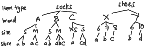
We can use a hierarchical approach to tackle both problems, but this approach is particularly needed in case 2. For example, the hierarchy might be:
- item type (shoes / socks / sandals)
- brand
- size
- store
Time series as a hierarchy
Note that although it’s frequently called as “hierarchy”, the following approaches are also applicable for grouped time series – they do not have to be in a hierarchical structure. There are some ways to approach this kind of problem.
1. Top-down approach
Here, we perform the forecast in the highest hierarchy level, let’s say, the item type. Then, these top-level forecast results are disaggregated into the lowest hierarchy level, either based on the proportion of historical sales quantity, or based on the proportion of the forecast values.
Pros:
- since the forecast is done on the top level, it works well despite having low values in the lower level hierarchy
- simple, easy to build
- provides a reliable forecast for aggregate levels
Cons:
- it is challenging to do the disaggregation accurately
- loses information about the dynamic series of the individual time series
2. Bottom-up approach
As described by its name, this approach forecast the values in the lowest hierarchy level, e.g., based on the combinations of item-brand-size-store. Then, we aggregate the forecast values to the top hierarchy level.
Pros:
- no loss of information because it incorporates the series on the lowest hierarchy level
- can capture dynamics of individual series
Cons:
- series in the lowest hierarchy level may have noisy data, e.g., a lot of zeroes
- requires a large number of series to be forecasted
3. Middle-out approach
This is a combination of the top-down and bottom-up approach. In this approach, we forecast in the middle hierarchy level, e.g., based on brands. Then, we do a top-down approach to disaggregate the values on the size-store level (either based on the historical or forecast proportion) and a bottom-up approach to aggregate the values into the item type.
4. Optimal reconciliation
In this approach, the forecast is done independently on each hierarchy level. As we might have expected, the results could be incoherent, for example, the total values based on item types are different from the total at the store level. To align the forecast values, a reconciliation approach is done using a linear optimisation method, such as ordinary least squares (OLS).
As quoted from [2]:
In summary, unlike any other existing approach, the optimal reconciliation forecasts are generated using all the information available within a hierarchical or a grouped structure. This is important, as particular aggregation levels or groupings may reveal features of the data that are of interest to the user and are important to be modelled. These features may be completely hidden or not easily identifiable at other levels.
Notes
At the moment, the hierarchical time series forecasting implementation is provided in hts package in R. I found a Python implementation in scikit-hts package, but it is still in the alpha version.
I haven’t created a proper case study on this example yet (my bad!). I did some trials using scikit-hts, but it requires a wide data format that defines the combination of hierarchy levels – a bit different from my usual long data format. However, there are a couple of example notebooks by the authors here.
Currently, I only have used the bottom-up approach while working on time series forecasting problems. I have experienced a problem as in Case 1, which is much easier because we can do the forecast at the top level without the needs for disaggregation. I will write another post once I’m more comfortable with the optimal reconciliation strategy.
References
[1] 10.1 Hierarchical Time Series - Forecasting: Principles and Practice. (n.d.). OTexts. https://otexts.com/fpp2/hierarchical.html
[2] 10.7 The optimal reconciliation approach - Forecasting: Principles and Practice. (n.d.). OTexts. https://otexts.com/fpp2/reconciliation.html
[3] https://github.com/carlomazzaferro/scikit-hts
[4] Panagiotelis, A., Athanasopoulos, G., Gamakumara, P., & Hyndman, R. J. (2020). Forecast reconciliation: A geometric view with new insights on bias correction. International Journal of Forecasting, 37(1), 343-359.
[5] Forecasting hierarchical time series. (2013, October 10). SlideShare. https://www.slideshare.net/hyndman/hierarchical
[6] Burba, D., & Chen, T. (2021). A Trainable Reconciliation Method for Hierarchical Time-Series. arXiv preprint arXiv:2101.01329.