When a straight line goes wrong

What score will John get if he studies for five hours before the exam?

You might be familiar with this kind of question in your math class. You have a list of students with their study duration and exam score, and you’re asked to estimate John’s score. In the example below, we can fit a line based on the data (black points) and predict John’s score. Simple, isn’t it?

Figure 1. Sample case: predicting exam score based on study duration. The red line depicts the predicted score.

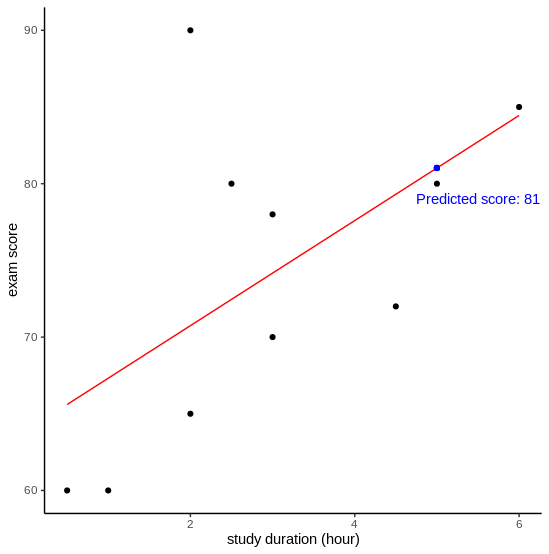
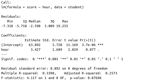
To come up with the regression line, we seek a line that minimizes the error of predicting the actual data. Based on this model, average students who do not study at all can get 64 on their exam. Additional one hour of study increases 3.4 score on average, although it does not seem that study duration is a statistically significant aspect that associates with the exam score (p-value = 0.077).

Figure 2. Summary of the linear model. Duration of study is not a statistically-significant aspect to predict the exam score.

How do we know if it is a good model?

We can measure the performance of this model by calculating the prediction error \(e\):

\[e_{i} = y_{i} - \hat{y}_{i}\]

To know whether it is good or not, we compare the sum of squared prediction error (\(SS_{residual}\)) to the sum of squared error if we merely predict the values based on the mean (\(SS_{total}\)). Note that error is also called as residual.

\[SS_{residual} = \Sigma_{i=1}^{n} e_{i}^2\] \[SS_{total} = \Sigma_{i=1}^{n}(y_{i} - \bar{y})^2\]

Then, we compute the \(R^2\). We can interpret \(R^2\) as percentage of variation in the data that is explained by the model. The value normally ranges from 0 to 1. If it is closer to 1, it means the model can capture the variation well. In some cases we might get negative \(R^2\), which means the model performs much worse than just predicting using the mean value.

\[R^2 = 1 - \frac{SS_{residual}}{SS_{total}}\]

In our model, \(R^2 = 0.34\). Although it is quite far from 1, we should not expect to find the “ideal” \(R^2\) while dealing with real-world data.

“Some fields of study have an inherently greater amount of unexplainable variation. In these areas, your \(R^2\) values are bound to be lower. For example, studies that try to explain human behavior generally have R2 values less than 50%. People are just harder to predict than things like physical processes.” [1]

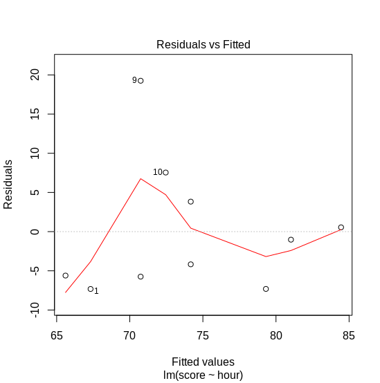
Aside from \(R^2\), we should also assess if the model is appropriate to fit the data we deal with. Simple linear model like in Figure 1 assumes that the prediction error is normally distributed, and it is homoskedastic. What does it mean?

Observing the error distribution

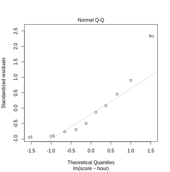
Based on the model we have, we can plot the fitted values vs. the residuals. We expect that the error has a constant variance, i.e., homoskedastic. As seen on Figure 3, the variance on exam score between 70 and 75 is higher than others. Additionally, we can observe the distribution of the residuals. Figure 4 shows a normal Q-Q plot: the x-axis shows the quantiles of error from our model. If the error is normally distributed, we expect them to follow the dotted line. Here, we observe that the error does not follow normal distribution. What should we do?

Figure 3. Fitted vs. residual plot of linear model in Figure 1

Figure 4. By looking at the normal Q-Q plot, we find that the error does not follow normal distribution.

Introducing generalized linear model

Let’s take a step back and rethink about our problem. We are trying to predict exam score based on duration of study (in hour). Based on our knowledge, we know that exam score is bounded in range 0 to 100. Additionally, duration of study is a positive integer. If we take these as considerations, our previous model does not make sense, since we can extrapolate the line until the score exceeds 100, and we also can put negative study duration. Uh, oh.

In these cases, we can use a generalized linear model. What is it? Simple linear models are written in this form:

\[y = \beta_{i} x_{i} + \epsilon\]

Since the value of \(y\) is bounded, we should find a function that connects the linear predictors to the outcome variable properly. This function is known as link function.

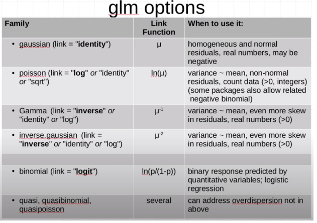
\[y = f(\beta_{i} x_{i} + \epsilon)\]

There are some link functions, which are dependent on the assumed error distribution (Figure 5). Simple linear model assumes the error is normally distributed (Gaussian family), and the link function is “identity”. Thus, if we build a generalized linear model (GLM) with that configuration, the result equals to a simple linear model. In this case, we can assume that the error follows binomial distribution, by viewing the score as a success (if score = 100) or failure (if score = 0) – this model is also called logistic regression. Figure 6 shows the model summary.

Figure 5. Available options of error distribution and the link functions in glm command (R) [2].

Since we use logit link, we should use inverse-logit function to transform the intercept’s estimate (\(\eta\)) and get the average exam score.

\[p = \frac{exp(\eta)}{1+exp(\eta)}\]

This model shows that on average, students get 62.72 on their exam. We also can interpret the estimates of covariates as an odd ratio. For instance: if a student studies for one additional hour, he/she is likely to get \(exp(0.18591) = 1.2\) times higher score than the average students.

Figure 6. Logistic regression model summary. In this model, hour is statistically significant.

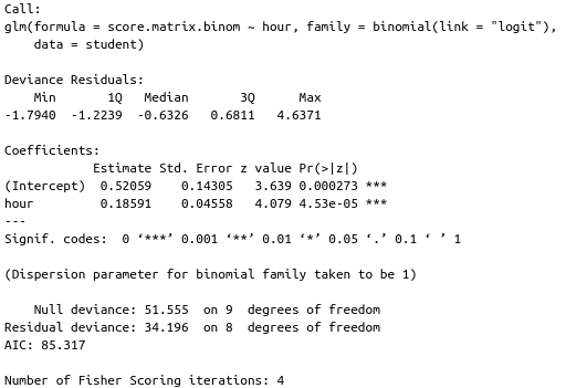
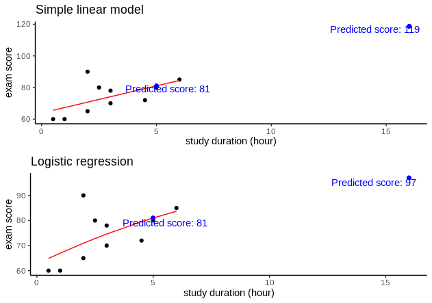
GLM function does not return \(R^2\), but we can calculate them based on the null deviance (\(SS_{total}\)) and residual deviance (\(SS_{residual}\)). Although the \(R^2 = 0.3367\), which is slightly lower than the linear model, this model is more reasonable to use. Figure 7 shows the comparison of predicted values when a student studies for 16 hours (Is this guy truly hard-working or do we have erroneous data?).

Figure 7. When we extrapolate the prediction, the simple linear model results in an unreasonable score. Meanwhile, logistic regression model seems more plausible in this case.

Takeaways

This post gives a short introduction of the generalized linear models. The selection of the family of distribution and logit link depends on the data we’re dealing with. Anyway, I want to emphasize that we should determine which distribution to use by looking at the distribution of error, not the original values. The “strategy” of determining the distribution by looking at histogram of the outcome variable is called histomancy [3]. For those who are keen to explore more, I recommend to read [3].

References

[1] How to interpret R-squared in regression analysis. (2019, May 30). Statistics By Jim. https://statisticsbyjim.com/regression/interpret-r-squared-regression

[2] Methods in Experimental Ecology I. (2016, November 5). Generalized Linear Models I. YouTube. https://www.youtube.com/watch?v=G5xIFdLL5Ic

[3] McElreath, R. (2018). Statistical rethinking: A Bayesian course with examples in R and Stan. CRC Press.