k-nearest neighbours explained

k-nearest neighbours (knn) is one of the most common algorithm in classification task. Actually, it also can be used to solve regression problem. To understand it in more detail, let’s proceed to the readings.

Note: this post is my written summary based on [1]

Intuition

Suppose we want to identify someone’s gender based on his/her height and weight. If there is a new person with height = 165 cm and weight = 62 cm, should we call that person as a he or she?

Figure 1. What is that person's gender?

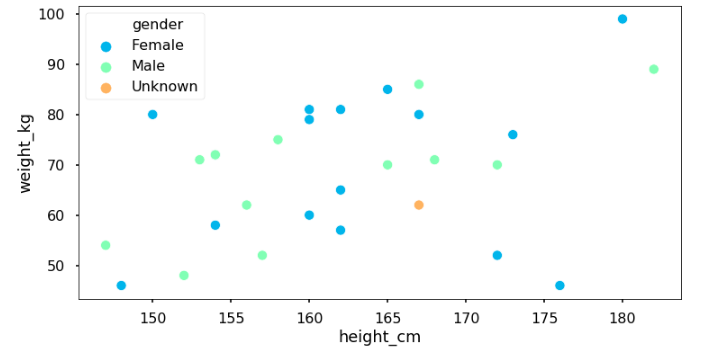
Here, we have set of points containing height and weight $(x, y)$. While Naive Bayes uses prior probability and Decision Tree computes information gain, k-nearest neighbours calculates proximity of the new point to other point.

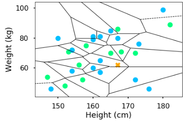
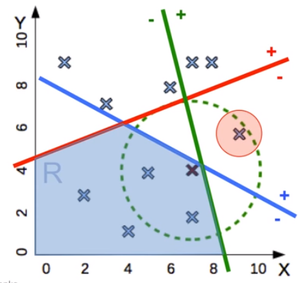
Using that intuition, we find the most similar point and use that point’s class as the prediction. Every training data point has its region around it, which is form of Voronoi tessellation. If a new point exists on certain region, it means that point has similar class to that region’s data point.

Figure 2. Decision boundary of each point

Thus, the new point is more similar to the blue point $(162,65)$ - which is a female.

Reflecting from the regions, knn has non-linear decision boundaries - unlike Decision Tree, Logistic Regression, or Naive Bayes. As a simple method, knn produces highly complex decision boundary.

Although it is quite simple, there are some drawbacks:

1. It is sensitive to outliers
   • A tiny change of the training set could make huge change to the decision boundary.
2. There is no confidence $P(y|x)$
   • knn doesn’t have notion of prior; it’s insensitive to class prior

To fix those drawbacks, we could use more than 1 nearest neighbour - then use majority vote to determine the prediction.

Algorithm

Classification

Given:

1. training examples ${x_i, y_i}$, where
   • $x_i$: attribute values
   • $y_i$: class label
2. testing point $x$

The training and testing set are used at the same time - there is no training phase in knn. It’s also called as instance-based learning.

Algorithm:

1. Calculate distance $D(x,x_i)$ to every training example $x_i$
2. Select $k$ closest instances $x_{i_1} … x_{i_k}$ and their labels $y_{i_1} … y_{i_k}$
3. Set the output class $\hat y$ based on the most frequent class in $y_{i_1} … y_{i_k}$

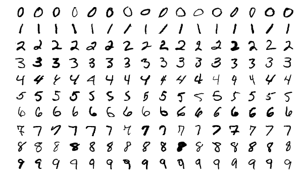
One of the well-known application of knn is handwritten digit classification on MNIST dataset. The dataset contains image of handwritten digits in 16x16 bitmaps, with 8-bit grayscale. To determine the distance of each image, we calculate distance of each pixel on pair of images using Euclidean distance:

$D(A,B) = \sqrt{\sum_r{\sum_c(A_{r,c}-B_{r,c})^2}}$

where $r$ equals to row and $c$ equals to column of pixel location in the image.

Figure 3. MNIST dataset (Source: Wikipedia)

Regression

On regression task, knn has similar algorithm with classification. Given:

1. training examples ${x_i, y_i}$, where
   • $x_i$: attribute values
   • $y_i$: numeric value of the target attribute
2. testing point $x$

Algorithm:

1. Calculate distance $D(x,x_i)$ to every training example $x_i$
2. Select $k$ closest instances $x_{i_1} … x_{i_k}$ and their labels $y_{i_1} … y_{i_k}$
3. Set the output value $\hat y$ based on the mean of $y_{i_1} … y_{i_k}$
   • $\hat y = f(x) = \frac{1}{k} \sum_{j=1}^{k}y_{i_j}$

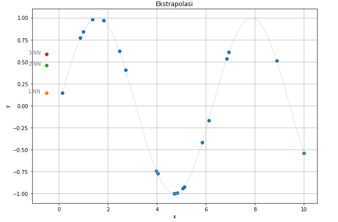
Suppose we have the blue points as training set, and we want to know y-value of a new data point $(6.5,y)$. Using 1-nn, we estimate its value equal to point $(7,0.55)$. If we use more nearest neighbours, we could observe how the predicted value changes.

Figure 4. Interpolation on knn regression (Source: [2])

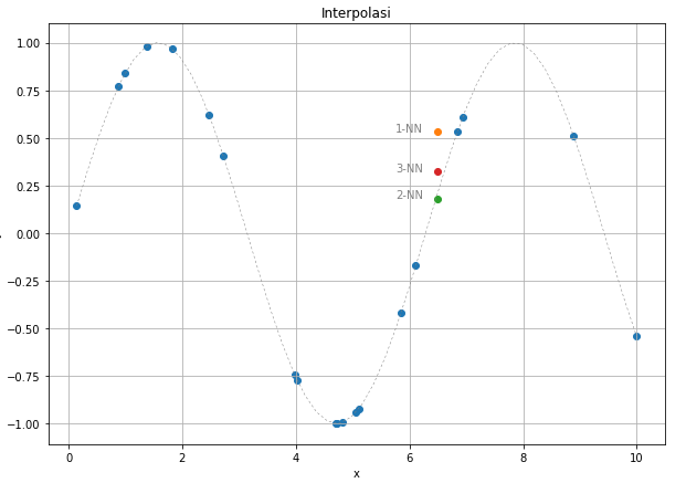
While it has decent performance if we use it to predict testing data which are still within the range of training set, we should be careful on using this to predict data outside the training set. As we can see on Figure 5, we couldn’t get y-value which fits sine wave on testing point $(-0.5,y)$. Remember that knn is an instance-based learner.

Figure 5. Extrapolation on knn regression (Source: [2])

Things to consider

How to choose value of $k$?

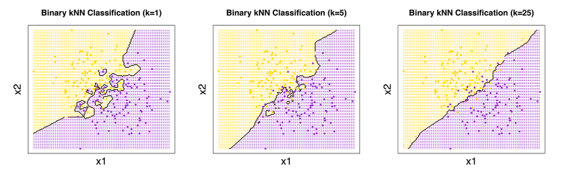
Our prediction result relies heavily on the value of $k$.

• If $k$ is too small, the model will have high variance and unstable decision boundaries
• If $k$ is too large, the model will classify everything as the most probable class $P(y)$

Thus, we should split the training set into a validation set. We validate the prediction result on validation set using different value of $k$, and choose model with $k$ value with the best performance.

Figure 6. How k affects decision boundary (Source: [3])

Which distance measure should be used?

Aside of $k$, distance function also highly affects the prediction result. Common distance measure used on continuous data is Euclidean distance. Euclidean distance treats all dimension equally, and is sensitive to extreme difference in single attribute.

Euclidean distance can be generalized into Minkowski distance (p-norm): $D(x_d,x’_d) = \sqrt[p]{\sum_d{|x_d-x’_d|}^p}$ Note: Euclidean distance has p = 2.

We could compare distance on categorical data using Hamming distance - it calculates number of attributes where $x$ differs with $x_i$.

Practical issues

Since we use majority vote to determine prediction result of classification task, the model could result in tie break: the neighbours are split into more than 1 class. We could avoid this by selecting odd number of $k$ - but this doesn’t resolve the problem if the case is multi-class.

To break the ties, we could do any of these approaches:

1. pick the class randomly: flip a coin to determine positive or negative class
2. prior: pick class with greater probability
3. conduct 1 nearest neighbour and use its class as prediction result

We should also take note that knn requires us to fill missing values on the dataset; and also make sure that each dimension has similar scale. It is crucial since the data are used to calculate the distance.

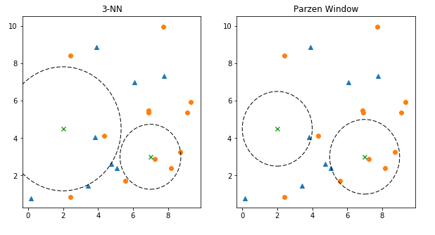
knn vs Parzen Window

knn has similar approach with Parzen Window, the difference is that knn select $k$ nearest neighbours to determine its decision boundary. Meanwhile, Parzen Window selects a constant-valued radius - all points within that radius are considered as the neighbours.

Figure 7. Difference between knn and Parzen Window (Source: [2])

Pros and cons

Pros:

• use almost no assumptions of the data, we only need to determine $k$ and the distance measure
• easy to update in online setting: we only need to add new item to the training set

Cons:

• need to handle missing values
• sensitive to outliers and mislabeled training data
• sensitive to irrelevant attributes, since it affects the distance calculation
• is computationally expensive:
  • space: need to store all training examples
  • time: need to calculate distance to all examples –> $O(nd)$, where $n$ = number of training set and $d$ = cost of computing distance
    • the computation is heavy on testing set ($O(nd)$), not on training ($O(d)$)

How to make knn faster

Since the complexity is $O(nd)$ on the test set, we could reduce it by:

• reducing $d$: use dimensionality reduction techniques
• reducing $n$: don’t compare the test set to all training set

There are several approaches to reduce the $n$.

k-d trees

k-d trees can be used on low dimensional data with real-value. By using this, we could reduce the complexity to $O({d}*{ log}_2 n)$. Note that it could work only when $d«n$; and it could miss nearest neighbours which aren’t on the region.

k-d trees work by building binary trees from training data: we pick a random dimension, find the median, then split the data into two regions. We repeat this step until certain depth.

Figure 8. k-d trees limit the nearest neighbours search to certain region (Source: [2])

Locality-Sensitive Hashing (LSH)

Locality-Sentive Hashing (LSH) can be used on high dimensional data, either real-valued or discrete data. The complexity could be reduced to $O(n’d)$ where $n’«n$.

LSH works similar to k-d trees, except that it splits the regions not based on median, but using random hyperplanes $h_1…h_k$. Each hyperplane split the region, which results in $2^k$ regions. Then, we select the nearest neighbours which reside on the same region as the testing point. That’s why it could miss the actual nearest neighbours.

Figure 9. Example of LSH (Source: [1])

Inverted list

Invested list can be used on high dimensional and sparse data, such as text. The complexity could be reduced to $O(n’d’)$ where $d’«d$ and $n’«n$; and the result is exact.

This approach is usually used on search engine to determine the most similar documents to a new document.

For example, we have set of documents:

• $D_1$: “give us food”
• $D_2$: “review more food to redeem voucher”
• $D_3$: “give review”
• $D_4$: “give donation”
• $D_5$: “more food review”
• $D_6$: “give voucher as donation”

Which document is more similar to the new document $D_6$? On inverted list, we merge the words of the documents and list down on which documents does each word exist.

• give: {1, 3, 4, 6}
• us: {1}
• food: {1, 2, 5}
• review: {2, 3, 5}
• more: {2, 5}
• to: {2}
• redeem: {2}
• voucher: {2, 6}
• donation: {4}
• as: {6}

Since $D_6$ has similar words to $D_1, D_2, D_3, D_4$, those documents can be identified as the nearest neighbours.

Conclusions

Having a comprehensive explanation of how k-nearest neighbours work, we understand why it is quite easy to use: we don’t need to specify lots of assumptions and it could work well on large dataset. However, the major drawback of this algorithm is its computational cost. Although there are several approaches to fasten its computation, we should put some things as considerations such as:

• is the dataset continuous or discrete?
• is it acceptable to have less accurate result in order to maintain the computational complexity?

References

[1] Victor Lavrenko - k-Nearest Neighbor Algorithm

[2] Ali Akbar Septiandri - Data Mining Course

[3] Burton DeWilde - Classification of Hand-written Digits (3)