Introduction to changepoint analysis

One of my recommended personal finance book is The Barefoot Investor: The Only Money Guide You’ll Ever Need. As a barefoot investor, you are suggested to allocate your income into several buckets: 1) blow (expenses and some splurge money), 2) mojo (safety money) and 3) grow (long-term wealth). Although I’ve unconsciously performed similar budgeting like this before, this book gives a wider perspective on money management, especially if you’are aiming to achieve financial freedom as soon as possible.

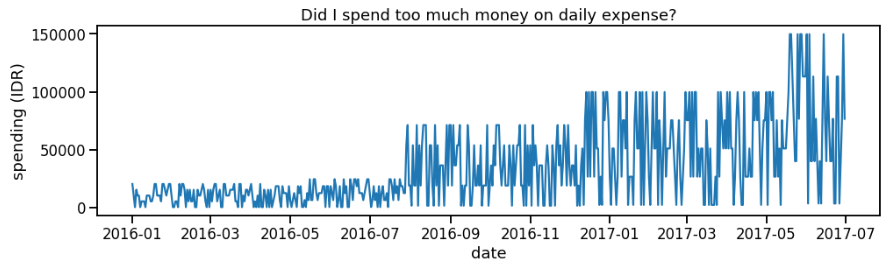
No matter you’ve read this book or not, have you ever wondered whether your daily spending is decreased after you get any financial advice? If you are not sure how to make a conclusion based on your data, this might be a fruitful reading for you.

Intuition

Welcome to change point analysis. As obvious as its name, it is a technique to identify whether there is any change in your data; and to find when the change occurs. Although it sounds simple, we tend to use our gut feeling and are prone to our subjective bias.

Figure 1. There's obvious increase, but how do we teach a computer to find it?

Techniques

There are two main types of change point analysis: offline and online analysis. When we use offline analysis, we process the data in batches and analyze the data in one go. This approach ends up with a more accurate results. On the other hand, online analysis is usually conducted when we analyze streaming data, where we aim to get the quickest results to identify when any changes start to occur. Based on this explanation, we can say that we are doing offline analysis while observing our daily expenses.

Control charts

If you are familiar with business process improvement, you might have used the control charts. To create a control chart, you should calculate the mean value of the observation, as well as the standard deviation. Then, you determine the upper and lower control limit (e.g. $\mu \pm2\sigma$). If an observation exceeds or is less than the control limit, we can say that the observation is out of the usual pattern.

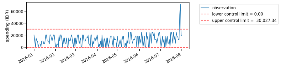
Let’s say that we analyze the data periodically in batches. Since we calculate the point-wise change based on the control limit, where the control limit is subject to the historical observations, we might have different conclusions when we observe the data on different period.

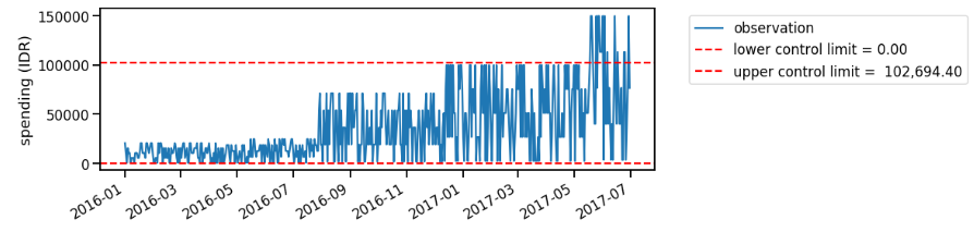
On Figure 2, we find unusual spike close to August 2016. However, as we obtain more data points, our control limit definition changes, and we no longer assume that the August 2016’s point as unusual (Figure 3). Well, my average spending is probably increased on that point since I’ve already worked on full time job, right?

Figure 2. Woah, there's a spike!

Figure 3. Previous spike (Figure 2) seems pretty normal now, eh?

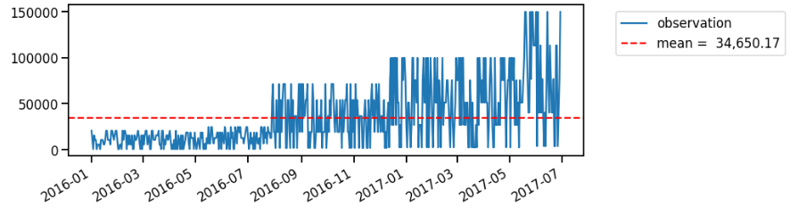
While control charts focus on point-wise change, you might be more interested in identifying the change of the mean. This is the time to use change point analysis! On this post, I’ll cover the simplest methods to do single change point analysis.

Cumulative sum (CUSUM) approach

CUSUM approach is quite simple:

1. Calculate mean value of all observations ($\hat{y}$)
2. Calculate residuals between each observation to the mean ($\epsilon_{i} = y_{i} - \hat{y}$)
3. Set cumulative sum of residuals at time 0 to zero ($S_{0} = 0$)
4. Calculate the cumulative sum of the residuals ($S_{i} = S_{i-1} + \epsilon_{i}$)
5. Plot the cumulative sum at each time

Figure 4. Let's plot the mean to make it more intuitive

Figure 5. Sample CUSUM plot. Observe the shape!

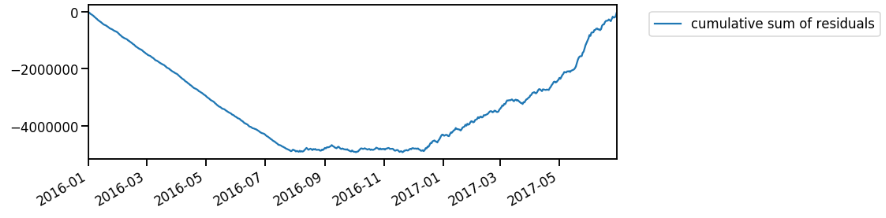
The CUSUM plot could show upward or downward trend. The upward trend describes that the period has higher value than the overall mean, while the downward trend shows that the period has lower value. When the trend turns into the opposite direction, it resembles the time when the change occurs.

Based on Figure 5, we could infer that up to August 2016, my spending is much lower than the overall mean. The first change point can be found after that, where the CUSUM plot shows rather steady line (there isn’t any significant changes). Meanwhile, the second change occurs around December 2016: the CUSUM plot shows increasing trend up to the last data point. It describes that the spending is much higher than the overall mean. I should’ve read money management book before, duh!

To analyze difference between the means of period before and after the change point, we can simply subtract the average value. However, CUSUM plot uses frequentist approach, where we gain confidence level by collecting data and observing the results in the long run. Since we have limited data points, we could use sampling without replacement, or in other words, we try to recreate new dataset by randomly reordering the observations. Steps:

1. Determine number of iterations $N$
2. For each iteration:
   • take random sample without replacement from the observations \(X^0_{1}, X^0_{2}, ..., X^0_{n}\), where $n$ = number of observations
   • calculate the sample’s cumulative sum of residuals ($S^0$): \(S^0_{1}, S^0_{2}, ..., S^0_{n}\)
   • calculate the difference between maximum and minimum residuals in each bootstrap \(S^0_{\text{diff}} = S^0_{max} - S^0_{min}\)
   • if \(S^0_{\text{diff}} < S_{\text{diff}}\), it means the result from the sample is consistent with the actual observations
3. Calculate confidence level: $\text{confidence level} (\%) = 100 * \frac{X}{N}$
   • where $X$ represents number of iteration which has \(S^0_{\text{diff}} < S_{\text{diff}}\)

In this example, apparently we are 100% confident that the change does exist.

Mean Squared Error (MSE) estimator

In this approach, we aim to identify structural change in the data, by estimating the changes based on the mean squared error. The intuition is, we try to find the time $k$ which is the best split of the data. When we observe the “best split”, it implies that the splitting results have the least similar observations, which happens due to the change.

Here are the steps:

1. Split the observations into two segments:
   • segment 1 = \(\left\{ 1, ..., m \right\}\)
   • segment 2 = \(\left\{ m+1, ..., n \right\}\)
2. Calculate average value of each segment: $\bar{X}_1$ and $\bar{X}_2$
3. Observe how well the observations fit to the estimated averages: \(MSE = \Sigma_{1}^{m}(x_{i} - \bar{X}_1)^2 + \Sigma_{m+1}^{n}(x_{i} - \bar{X}_2)^2\)
4. Value of $m$ which minimizes the mean squared error is the best estimate of last point before the change occurred

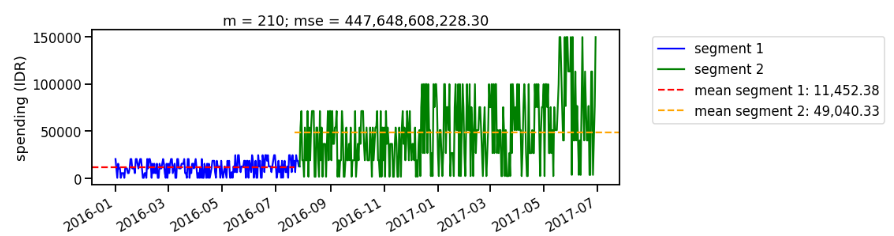
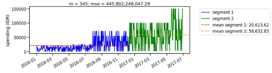
As we iterate the segmentation, we look for segment with the lowest mean squared error. For example, when we split the data on the 210th day (around August 2016), we still find large mean squared error on the second segment (Figure 6). Iterating the segmentation multiple times, we find the best split occurs around December 2016 (Figure 7). The result is consistent with what we observe using CUSUM approach.

Figure 6. Not the best split

Figure 7. The mean changes in the end of December 2016

Conclusions

As we already learned, change point analysis methods help us to teach computers (or even ourselves) how to identify whether any changes occur. The approaches I shared above can be implemented on your own easily, you can find the sample code here. However, don’t stop here, as there are more change point analysis methodologies to explore! You can start by learning from the available libraries, such as bayesloop in Python or changepoint package in R.

References

[1] Change-Point Analysis: A Powerful New Tool For Detecting Changes

[2] Change Point Analysis