
Have you ever wondered how much money you would spend if you didn’t start smoking last year? Have you imagined how relieved you would be if you managed to say sorry after being rude to your parents? Sometimes we want to know the effect of our decision, but unfortunately we can’t observe the alternate universe - condition when we don’t take such decision. Thus, how could we know whether we took the right decision or not?
On these cases, we can do time series hypothesis tests. Wait, what is it? Let me give a little explanation..
- Time series: set of data which are obtained in sequential order, and are composed of components like trend and seasonality. For example: daily household spending, transaction value of a grocery store.
- Hypothesis test: examination whether the observed data support our initial guess, e.g. team A plays better than team B.
In brief, time series hypothesis testing talks about how we identify whether different time periods have significantly different observation. What’s the difference with conducting t-test? Well, we indeed compare difference between two or more groups; but the challenge is that each observation on time series data has serial dependency to other observations, also contains trend and seasonality (e.g. transactions grow 1.5x over past 3 years, more transactions occur on weekends), so we can’t simply separate the observation into some groups.
We use two approaches here:
1. Time Series Hypothesis Test
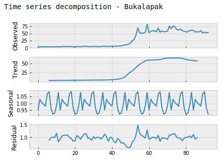
As previously stated, time series data has autocorrelation - serial dependency with previous data points; which means we couldn’t directly split the data into two groups and compare them. By removing trend and seasonal components from the data, we have residuals of the series. If the residuals fulfill normality assumption (i.e. the residuals are normally distributed), we can proceed to hypothesis test. Initially, we should define the null hypothesis - the one hypothesis we try to reject.
To gain more understanding, we use Bukalapak search query data as the case study: we want to check whether number of search query is significantly different after Bukalapak Nego Cincai campaign release. The notebook can be accessed here.
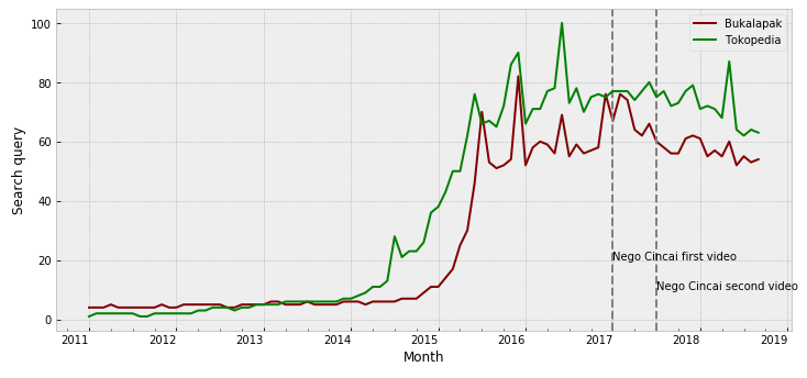
Note: Tokopedia’s search query will be used later; we can see that it has similar trend with Bukalapak, with earlier increasing popularity.
We conduct two hypothesis tests:
Test 1:
- H0: there is no difference between number of search queries before and after first campaign
- H1: number of search queries before first campaign is different with after campaign
Test 2:
- H0: there is no difference between number of search queries before and after second campaign
- H1: number of search queries before second campaign is different with after campaign
We use two sample t-test; we want to know whether average of each group (period) is significantly different with the other group. The main idea of t-test is trying to check whether the observed value (signal) is stronger than the variation on the data (noise). If the signal is stronger than the noise, it is more likely to observe statistical significance. How does it work?
First, we calculate mean of observation on each group, then subtract them to get the mean difference (the “signal”). Then, we calculate the variance of each group, and calculate pooled standard deviation: weighted average of variation within each groups (the “noise”). The “signal” is divided by “noise” to obtain the t-value; higher t-value means it is more likely to observe statistical significance (lower p-value). The formula isn’t elaborated here, but you can refer to the first and second link on Reference section.
From both tests, we fail to reject the null hypotheses with p-value on test 1 = 0.448 and test 2 = 0.611; thus we could infer that there is no significant effect of the campaign.
2. Causal Impact Analysis
While t-test could be used on time series data, we might get overoptimistic inferences since the residuals might still have autocorrelation each other, thus violates independence assumption. Alas, it is more suitable to use causal impact analysis. On this approach, the original time series and another control time series are used to construct a model. The model will predict observation of the “alternate universe”; we can measure the impact of the actual decision by subtracting actual observation with the prediction. CausalImpact package is a really helpful package, by the way.
Again, we conduct two tests, to check significance of first and second campaign. We use Tokopedia’s search query as additional model components, especially since it has similar trend and seasonality with Bukalapak’s (Figure 2), so we can use it as control group.
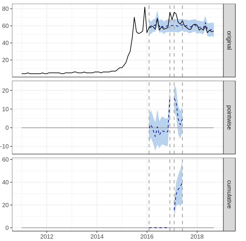
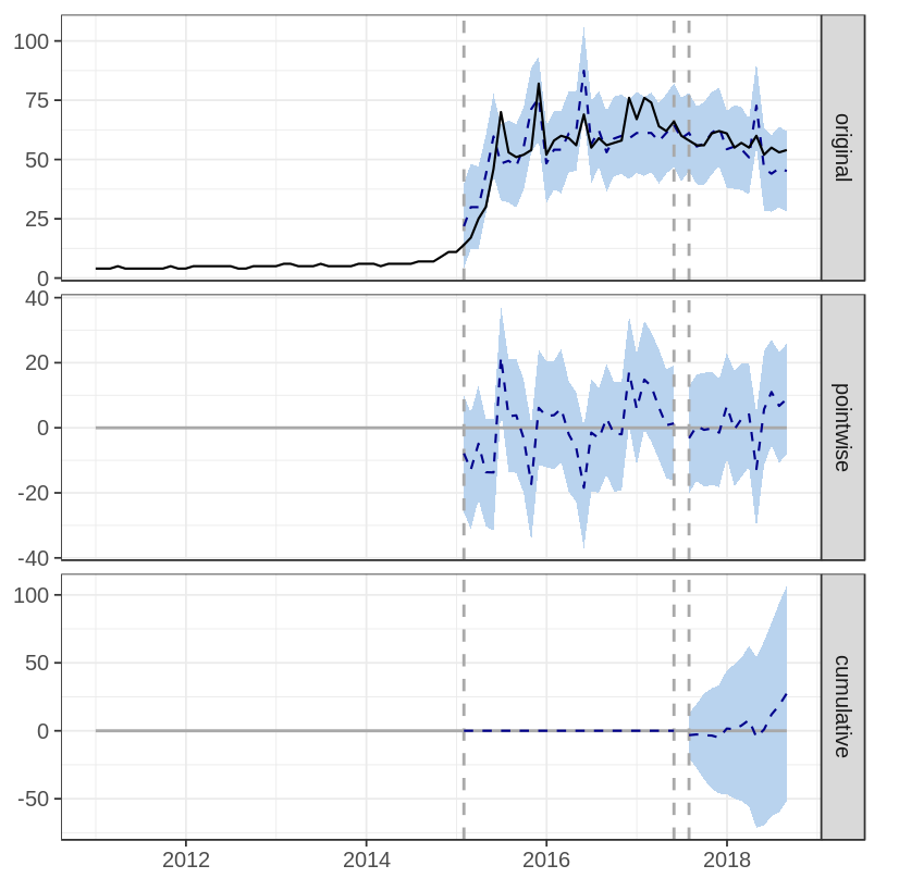
There are three plots on CausalImpact’s output:
- original: shows actual observation (solid line) and the prediction (dashed line)
- pointwise: shows difference between predicted and actual value per data point
- cumulative: shows cumulative difference between predicted and actual value
The first campaign shows increasing search query compared to the prediction (when no campaign is released), and the impact is statistically significant with p-value = 0.001. Meanwhile, second campaign doesn’t seem to have any effect on the search query (p-value = 0.254). Detailed result can be seen here.
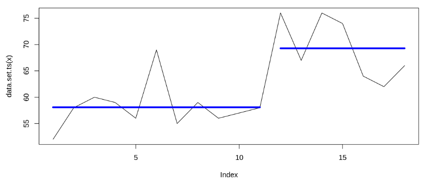
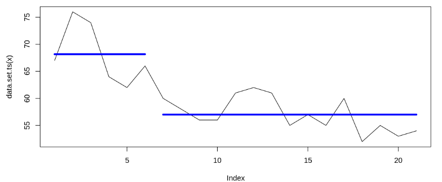
Since result of two sample t-test and causal impact differs, we use Bayesian change point as final check.
Extra: Bayesian change point
Based on the data (for test 1 and test 2), we try to estimate on which point of time the data changes. It appears that the change point occurs on January and July 2018 (when the first and second campaign started). Detected change point on January 2018 supports causal impact analysis’s results; while although we observe change point on July 2018, causal impact analysis shows that the difference isn’t statistically significant. Thus, we can infer that the first campaign significantly increases Bukalapak’s search query; while the second campaign doesn’t.
Conclusions
As long as we have data, it is not impossible to evaluate effect of our decision. I recommend using causal impact analysis rather than t-test, since t-test might give us overoptimistic approach. Bayesian change point analysis can also help on finding the point(s) where the observation started to change.
Aside from these approaches, convergent cross mapping can also be used to detect causality between time series - I haven’t explored it, though.
References
[2] iSix Sigma - Making sense of two sample t-test